
Problem Description
The Rubik’s cube is a three-dimensional combination puzzle invented by Emo Rubik in 1974. The physical version of the Rubik’s cube consists of small blocks that rotate on a central axis. Classically, the puzzle has six faces, each with nine blocks arranged in a \(3 \times 3\) square. More complicated versions of the Rubik’s cube exist with \(N \times N\) faces. Each block has a colored sticker in either white, red, blue, orange, green, or yellow. To solve the puzzle, the player must rotate one strip of blocks at a time until each of the six faces of the cube is populated by a single color.
Every year, dozens of Rubik’s cube competitions are held around the world in which the objective is to solve the puzzle as fast as possible. A number of easily memorizable algorithms exists that allow players to solve any Rubik’s cube configuration. However, solving these puzzles is not just of interest to players. There is also much academic interest in designing efficient algorithms to solve a Rubik’s cube in as few turns as possible.
The goal of this case study is to present a mixed-integer program that can solve an \(N \times N \times N\) Rubik’s cube from any starting configuration.
Methodology
Given any \(N \times N \times N\) Rubik’s cube, a unique set of \(m\) moves exists. It is important to note that moves are a sequence that involves many position-to-position mappings. We define moves to be quarter-turns of a block strip in either direction; half-turns require two moves.
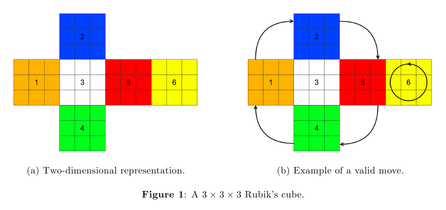
Consider the two-dimensional representation of a standard \(3 \times 3 \times 3\) Rubik’s cube in Figure (1). In this figure, a rotation of face 6 of the cube also rotates a row in the four neighboring faces. It is easy to verify that all moves can be exhausted by taking any face and considering all row- and column-wise turns, and then taking one vertically (horizontally) adjacent face and considering all row-wise (column-wise) turns. With the standard \(3 \times 3\ \times 3\) cube, this yields 18 unique moves. More generally, this yields \(6N\) unique moves for an \(N \times N \times N\) cube.
Notation
Notation used to define the model are introduced below.
- \(N\) denotes the number of faces on the Rubik’s cube (for this case study, we assume \(N = 3\)).
- The faces of the Rubik’s cube are indexed by \(f = 1, \ldots, 6\).
- Let \(r, c = 1, \ldots, N\) index the rows and columns, respectively, of each face. The tuple \((f,r,c)\) is a fixed position on the Rubik’s cube.
- The function \(x(f,r,c,t)\) defines the color of the block in position \((f,r,c)\) on turn \(t\). As there are six faces, \(x(f,r,c,t)\) can take on values one through six, representing the six colors of the cube.
- Let \(A(f,r,c)\) denote the set of moves associated with position \((f,r,c)\); that is, the set of moves that involve the block in position \((f,r,c)\) moving, and consequently being replaced by a new block. Thus if move \(m \in A(f,r,c)\) is made on turn \(t\), \(x(f,r,c,t) = x(f_m, r_m, c_m, t+1)\), where \((f_m,r_m,c_m)\) is the new position of the block originally occupying position \((f,r,c)\) after move \(m\).
Computing all possible moves for Rubik’s cube
Given our framework, a set of heuristics can be devised that generates all moves automatically for any \(N \times N \times N\) Rubik’s cube. Figure (2) is a snapshot of the code that produces the first \(3\) moves on a \(3 \times 3 \times 3\) cube.
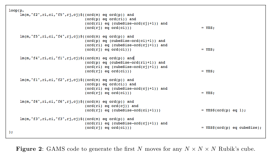
Variable \(p\) indexes either the rows or the columns. Let’s consider the case when \(p = 1\). lm(m,fi,ri,ci,fj,rj,cj) indicates that move \(m\) is associated with transfering the block in the initial position \((f_i,r_i,c_i)\) to the terminal position \((f_j,r_j,c_j)\).
- The first condition defining the set
ord(m) eq ord(p)assigns this mapping to the first (\(p = 1)\) move. - The second condition
ord(p) eq ord(ri)says that we are concerned with moving blocks in the first row of face 2. - The third condition
ord(ri) eq (cubeSize - ord(cj)+1)says that the last column of face 5 is the terminal location of the blocks from face 2 - The last condition
ord(rj) eq ord(ci)ensures that the row index of the initial position in face 2 matches the column index in the terminal position in face 5.
The rest of the code can be interpreted in the similar fashion. Combining all of these generates all moves displayed in Figure (1b). Counterclockwise quarter-turns move blocks from face 2 to face 5, from face 5 to face 4, from face 4 to face 1, and from face 1 to face 2. The fifth line of the code also defines the rotation of blocks within face 6 (when \(p = 1\)). The last line of the code describes the actions within face 3 (when \(p = 3\)). By turning the “middle” row of the cube, faces 3 and 6 do not change, but blocks within the other faces still rotate (when \(p = 2\)).
Given all possible legal moves for a Rubik’s cube, the set of move associations \(A(f,r,c)\) is constructed by computing within GAMS: bm_assc(m,f,r,c)=YES, which is equivalent to \(m \in A(f,r,c)\).
The Rubik’s Cube Model
Assuming that all moves and move associations can be generated, we now consider the solution of a Rubik’s cube. Given any \(N \times N \times N\) Rubik’s cube, we consider the following model:
\begin{align}
\min&\qquad\sum_t\sum_m y(m,t)\cdot t \\[5pt]
\text{subject to}&\qquad \sum_m y(m,t)\le 1\\[5pt]
&\qquad x(f,r,c,t)-M(1-y(m,t))\le x(f_{m},r_{m},c_{m},t+1)\\[5pt]
&\qquad x(f,r,c,t)+M(1-y(m,t))\ge x(f_{m},r_{m},c_{m},t+1)\\[5pt]
&\qquad x(f,r,c,t)-M\sum_{m\in A(f,r,c)}y(m,t)\le x(f,r,c,t+1)\\[5pt]
&\qquad x(f,r,c,t)+M\sum_{m\in A(f,r,c)}y(m,t)\ge x(f,r,c,t+1)\\[5pt]
&\qquad \sum_n z(f,r,c,t,n)\cdot n=x(f,r,c,t)\\[5pt]
&\qquad \sum_n z(f,r,c,t,n)=1\\[5pt]
&\qquad \sum_r\sum_c z(f,r,c,t,n)\ge N^2\cdot v(f,t,n)\\[5pt]
&\qquad \sum_r\sum_c z(f,r,c,t,n)+1\le N^2+v(f,t,n)\\[5pt]
&\qquad \sum_f\sum_n v(f,t,n)\ge 6\cdot d(t)\\[5pt]
&\qquad \sum_f\sum_n v(f,t,n)\le 5+d(t)\\[5pt]
&\qquad \sum_t d(t)\ge 1
\end{align}
The function \(x(f,r,c,t)\), which indicates the color of the block in position \((f,r,c)\) on turn \(t\), takes on integer values one through six; all remaining variables are binary:
- \(y(m,t)\) indicates whether move \(m\) is made on turn \(t\)
- \(z(f,r,c,t,n)\) indicates whether \(x(f,r,c,t) = n\)
- \(v(f,t,n)\) indicates whether every block on face \(f\) is color \(n\) on turn \(t\); and
- \(d(t)\) indicates whether the Rubik’s cube is solved by turn \(t\).
The model minimizes an objective value that is increasing in the number of turns taken and increasing in the time at which a turn is made. Thus, the model aims to solve the Rubik’s cube in as few steps as possible. The model constraints are described below.
Constraint 1: Constraint (1) ensures that no more than one move is made per turn.
Constraints 2 and 3: Assume \(M\) is chosen such that \(M \ge 5\). Constraints (2) and (3) together ensure that \(x(f,r,c,t+1)\) is between \(x(f,r,c,t) – M\) and \(x(f,r,c,t) + M\). Consider a move \(m \in A(f,r,c)\). If \(y(m,t) = 0\) (move \(m\) is not made on turn \(t\)), then the constraints leave \(x(f,r,c,t+1)\) unbounded. If \(y(m,t) = 1\), then the constraints ensure that \(x(f,r,c,t) = x(f_m,r_m,c_m,t+1)\) so that the block in position \((f,r,c)\) on turn \(t\) is moved to position \((f_m,r_m,c_m)\) on turn \(t+1\).
Constraints 4 and 5: If \(y(m,t) = 0\) for all \(m \in A(f,r,c)\), then the constraints force \(x(f,r,c,t) = x(f,r,c,t+1)\); that is, when no move is associated with position \((f,r,c)\) is made, then the block in position \((f,r,c)\) does not move. If \(y(m,t) = 1\) for some \(m \in A(f,r,c)\), then the constraints leave \(x(f,r,c,t)\) unbounded. When combined with constraints (2) and (3), the equations ensure that if a move \(m \in A(f,r,c)\) is made on turn \(t\), then \(x(f,r,c,t) = x(f_m,r_m,c_m,t+1)\); otherwise, if \(m \notin A(f,r,c)\) is not made on turn \(t\), then \(x(f,r,c,t) = x(f,r,c,t+1)\).
Constraints 6 and 7: Constraints (6) and (7) guarantee that \(z(f,r,c,t,n) = 1\) if and only if \(x(f,r,c,t) = n\).
Constraints 8 and 9: Constraints (8) and (9) define bounds on the number of blocks on face \(f\) with color \(n\) on turn \(t\). Thus, if \(v(f,t,n) = 1\), then all blocks on face \(f\) are color \(n\) on turn \(t\).
Constraints 10 and 11: The left-hand side of constraints (10) and (11) is equal to one if face \(f\) is complete, that is, if all blocks on face \(f\) have the same color, and zero, otherwise. The constraints state that the cube is solved (\(d(t) = 1\)) if all faces are complete.
Constraint 12: Constraint (12) states that the cube must be solved (i.e., \(d(t) = 1\) for some \(t\)).
The GAMS model is available for download here.
Some Results
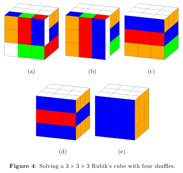
Figure (4) displays the results for the \(3 \times 3 \times 3\) cube defined in rubiks3x3.dat. The cube is sovled in four turns. In the first turn, Figure (4a) to (4b), the third row of the front face is quarter-turned to the left. In the second turn (4b) to (4c), the front face is rotated counterclockwise 90 degrees. In the third turn (4c) to (4d), the third row of the front face is quarter-turned to the right. Finally, in the last turn (4d) to (4e), the second row of the front face is quarter-turned to the left.
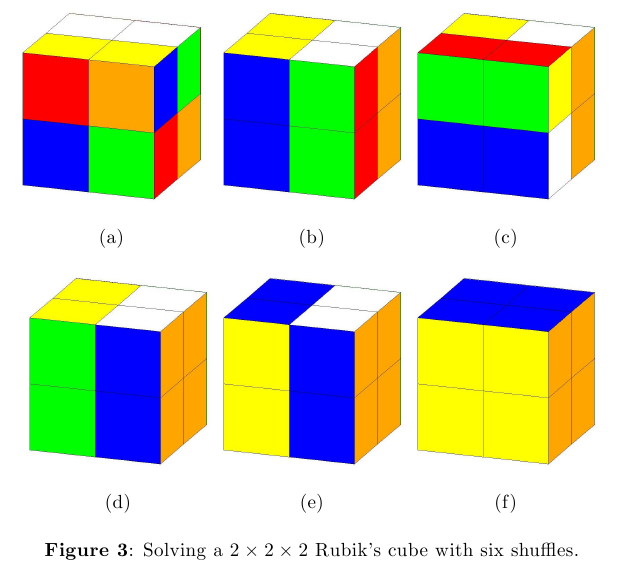
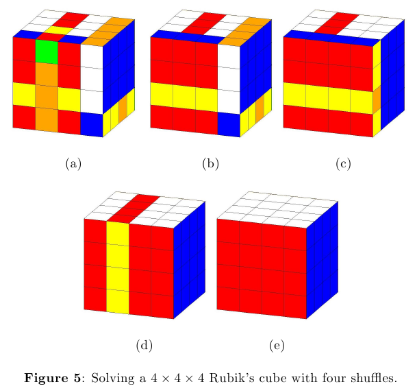
Figures (3) and (5) demonstrate the model on Rubik’s cubes of size \(2\times 2\times 2\) with 6 shuffles and \(4\times 4\times 4\) with 4 shuffles.
Limitations
The number of turns allotted \(T\) (length of set \(t\)) must be sufficiently large so that the model is solvable. For more complex cubes, larger values of \(T\) are needed to maintain model feasibility. It can be verified that for an \(N \times N \times N\) cube, the model can be solved for \(6T(7N^2 + N + ^6) + T\) variables. For a standard cube with \(N = 3\), this amounts to 433 variables per turn allotted. As a result, even for cubes with a single shuffle, larger values of \(T\) increase runtime substantially. Ideally, \(T\) should be the smallest value such that the model is solvable.
Supporting Scripts
The following Matlab scripts utilize Joren Heit’s Rubik’s Cube Simulator and Solver available for download from Mathworks.
To generate an NxNxN Rubik’s cube in the appropriate format for GAMS, run generateRubiks.m. To create the images for a given solution to a Rubik’s cube, use plotRubiksCube.m.
%%%%%%%%%%%%%%%%%%%%%%%%%%%%%%%%%%%%%%%%%%%%%%%%%%%%%%%%%%%%%%%%%%%%%%%%%%%%%%%
% Purpose: Creates data for NxNxN Rubik's cubes that can be fed into GAMS.
%
% Dependencies: Joren Heit's Rubik's Cube Simulator and Solver is used
% to generate a valid, random Rubik's Cube. This work can be found here:
% http://www.mathworks.com/matlabcentral/fileexchange/31672-rubik-s-cube-simulator-and-solver
%
% Inputs:
% -sizeCube:     The number of blocks to be in each row and column.
%                Ex: If sizeCube = 3, a 3x3x3 Rubik's Cube will be generated.
% -shuffleSteps: The number of random steps used to shuffle the cube.
% -turns:        The number of turns you want to give the mixed integer
%                program to solve the Rubik's cube.
%                Note: If you are choosing a lot of shuffle steps, you need
%                a high value of t, or else you risk infeasability.
% -directory:    The directory where you want your output file to be
%                stored. It's advisable to save your output file where you
%                run your GAMS files.
% -fileName:     Desired name of output file. This fileName will be concaten-
%                ated with an n x n suffix.
%                Ex: If fileName = rubiks and sizeCube = 3, the output file
%                will be titled rubiks3x3.dat.
%
%%%%%%%%%%%%%%%%%%%%%%%%%%%%%%%%%%%%%%%%%%%%%%%%%%%%%%%%%%%%%%%%%%%%%%%%%%%%%%%

function generateRubiksData(sizeCube,shuffleSteps,turns,directory,fileName)

    addpath Digital_Rubiks_Cube/src/;

    % Generate valid, random Rubik's Cube.
    generatedCube = rubgen(sizeCube,shuffleSteps);
    rubplot(generatedCube);

    % Create file suffix.
    fileNameSuffix = strcat(num2str(sizeCube),'x',num2str(sizeCube));

    % Output it to a file that GAMS can read.
    fid = fopen(strcat(directory,fileName,fileNameSuffix,'.dat'),'w');
    fprintf(fid,'sets\n');
    fprintf(fid,'\tf \"faces\" / f1 * f6 /\n');
    fprintf(fid,'\tr \"rows\" / r1 * r%d /\n',sizeCube);
    fprintf(fid,'\tc \"columns\" / c1 * c%d /\n',sizeCube);
    fprintf(fid,'\tm \"moves\" / m1 * m%d /\n',sizeCube*6);
    fprintf(fid,'\tt \"turns\" / t1 * t%d /\n',turns);
    fprintf(fid,'\tn \"color\" / c1 * c6 /;\n\n');
    fprintf(fid,'scalar\n');
    fprintf(fid,'\tcubeSize \"size of cube\" / %d /;\n\n',sizeCube);
    fprintf(fid,'parameters\n');
    fprintf(fid,'\tinitial_x(f,r,c) /\n');
    % The faces of the generated cube must be translated to match the way
    % they are expected to be input in the GAMS code.
    trans = [3 5 6 1 2 4];
    for i = 1:6
        for j = 1:sizeCube
            for k = 1:sizeCube
                if (i == 6 & j == sizeCube & k == sizeCube)
                    fprintf(fid,'\tf%d.r%d.c%d %d /;\n',trans(i),j,k,generatedCube(j,k,i));
                else
                    fprintf(fid,'\tf%d.r%d.c%d %d\n',trans(i),j,k,generatedCube(j,k,i));
                end
            end
        end
    end
    fclose(fid);

end
%%%%%%%%%%%%%%%%%%%%%%%%%%%%%%%%%%%%%%%%%%%%%%%%%%%%%%%%%%%%%%%%%%%%%%%%%%%%%%%
% Purpose: Plot GAMS output and save it to specified outDirName.
%
% Dependencies: Joren Heit's Rubik's Cube Simulator and Solver is used
% to generate a valid, random Rubik's Cube. This work can be found here:
% http://www.mathworks.com/matlabcentral/fileexchange/31672-rubik-s-cube-simulator-and-solver
%
% Inputs:
% -solFile:      The output file produced by GAMS.
% -sizeCube:     The number of blocks to be in each row and column.
%                Ex: If sizeCube = 3, a 3 x 3 Rubik's Cube will be generated.
% -outDirName:   What you would like the output folder in the working
%                directory to be called. For example, if outDirName =
%                rubiks3x3plots, you can find your results in a directory
%                called rubiks3x3plots in the working directory.
%
% Outputs: A directory called outDirName in which there will be images for
%          all steps of the solution.
%
%%%%%%%%%%%%%%%%%%%%%%%%%%%%%%%%%%%%%%%%%%%%%%%%%%%%%%%%%%%%%%%%%%%%%%%%%%%%%%%

function plotResults(solFile,sizeCube,outDirName)

    addpath Digital_Rubiks_Cube/src/;

    fid = fopen(solFile);

    tline = fgetl(fid);

    f1 = [];
    f2 = [];
    f3 = [];
    f4 = [];
    f5 = [];
    f6 = [];

    % Collect the solutions into 6 matrices, one for each face.
    while ischar(tline)
        formatSpec = '            %f            %f            %f';
        sizeFace = [sizeCube sizeCube];
        face = fscanf(fid,formatSpec,sizeFace);
        if (length(findstr(tline,'f1')) > 0)
            f4 = [f4 face'];
        elseif (length(findstr(tline,'f2')) > 0)
            f5 = [f5 face'];
        elseif (length(findstr(tline,'f3')) > 0)
            f1 = [f1 face'];
        elseif (length(findstr(tline,'f4')) > 0)
            f6 = [f6 face'];
        elseif (length(findstr(tline,'f5')) > 0)
            f2 = [f2 face'];
        elseif (length(findstr(tline,'f6')) > 0)
            f3 = [f3 face'];
        end
        tline = fgetl(fid);
    end

    % Generate a cube as a base.
    graphCube = rubgen(sizeCube,0);
    % Create the name base of the output file names.
    nameBase = strcat(num2str(sizeCube),'x',num2str(sizeCube),'c');
    % Determine how many plots will need to be made.
    plots = size(f1,2)/sizeCube;

    mkdir(outDirName);

    % Save each plot to the specified directory.
    for i=1:plots
        fileName = strcat(nameBase,num2str(i));
        graphCube(:,:,1) = f1(:,1:sizeCube);
        graphCube(:,:,2) = f2(:,1:sizeCube);
        graphCube(:,:,3) = f3(:,1:sizeCube);
        graphCube(:,:,4) = f4(:,1:sizeCube);
        graphCube(:,:,5) = f5(:,1:sizeCube);
        graphCube(:,:,6) = f6(:,1:sizeCube);
        f1 = f1(:,sizeCube+1:size(f1,2));
        f2 = f2(:,sizeCube+1:size(f2,2));
        f3 = f3(:,sizeCube+1:size(f3,2));
        f4 = f4(:,sizeCube+1:size(f4,2));
        f5 = f5(:,sizeCube+1:size(f5,2));
        f6 = f6(:,sizeCube+1:size(f6,2));
        figure1 = figure;
        rubplot(graphCube);
        set(gca,'position',[0 0 1 1],'units','normalized');
        saveas(figure1,[strcat(outDirName,'/') fileName '.jpg']);
    end

    fclose(fid);

end