
This Domino Artwork case study describes the optimization model that underlies the NEOS Domino solver, which constructs pictures from target images using complete sets of double-nine dominoes. Complete sets of double-nine dominoes include one domino for each distinct pair of dot values from 0 to 9. The NEOS Domino solver is an implementation of the work of Robert Bosch of Oberlin College.
Background Information
In his 2006 article “Opt Art”, Robert Bosch of Oberlin College describes some applications of optimization in the area of art. Domino artwork is a type of photomosaic, a picture made up of many smaller pictures. The small pictures can be seen up close but, at a distance, they merge into a recognizable image.
To create a photomosaic, we partition a target image and a blank canvas into a grid. Then, given a set \(F\) of building-block photographs, we place each photograph from \(F\) onto one square of the blank canvas grid with the goal of arranging the building blocks to resemble the target image as closely as possible. Optimization is well-suited to assigning the building blocks to the blank canvas grid but choosing the set of building blocks requires an artist’s touch!
Here, we describe domino artwork, which is a special type of photomosaic in which the building blocks are dominoes. The building-block set in the Domino solver is comprised of complete sets of double-nine dominoes; double-nine domino sets contain one domino for each distinct pair of dot values from 0 to 9.
Mathematical Formulation
In this section, we present Bosch’s integer programming model for constructing domino artwork images. Instead of a set of photographs \(F\), we have a set \(D=\lbrace d = (d_1, d_2): 0 \leq d_1 \leq d_2 \leq 9\rbrace\) of double-nine dominoes. Each domino \(d=(d_1, d_2) \in D\) is black with \(d_1\) dots on one square and \(d_2\) dots on the other square. The domino has a brightness value associated with each half; the value corresponds to the number of dots, so it is measured on a scale from 0 to 9, black to white.
Each domino can be positioned horizontally or vertically covering two squares of the canvas. A complete set of double-nine dominoes contains 55 dominoes, and exactly $s$ complete sets must be used. Therefore, we need to partition the target image and the canvas into \(m\) rows and \(n\) columns such that \(mn = 110s\).
The decision variable is a yes-no decision for each possible assignment of a domino \(d\) to a pair of adjacent squares of the canvas. This is more complicated than a yes-no decision associated with assigning a single photograph to a single square on a canvas. However, we can introduce a binary variable \(x_{dp}\) for each domino \(d \in D\) and each pair \(p \in P\) where \(P\) is defined as:
\[P = \big\{ \lbrace(i,j),(i+1,j) \rbrace : 1\leq i\leq m-1, i \leq j \leq n \big\} \\
\cup \big\{ \lbrace (i,j),(i,j+1)\rbrace : 1\leq i \leq m, 1 \leq j \leq n – 1 \big\}.\]
Associated with each assignment of a domino \(d\) to a pair of squares \(p\) is a cost \(c_{dp}\). The cost \(c_{dp}\) is calculated based on how close the dots of domino \(d\) match up with the brightness values of the target image. Let \(\beta_{ij}\in[-0.5,9.5]\) represent the brightness value of square \((i,j)\) on the grid representation of target image, and recall that \(d=(d_1,d_2)\) represents a domino with \(d_1\) dots on one square and \(d_2\geq d_1\) dots on the other square. An explicit expression for \(c_{dp}\) with \(p=\lbrace (i_1,j_1), (i_2,j_2)\rbrace\in P\) is
\[c_{dp} = \min\lbrace
\left(d_1-\beta_{i_1j_1}\right)^2 + \left(d_2-\beta_{i_2j_2}\right)^2,
\left(d_1-\beta_{i_2j_2}\right)^2 + \left(d_2-\beta_{i_1j_1}\right)^2
\rbrace.\]
The cost is calculated by adding the squares of the differences between dot values and actual brightness values for each orientation. \(c_{dp}\) becomes the minimum of these values.
Then, the domino optimization model can be written as:
\[\begin{array}{rrcll}
\text{minimize} & \sum_{d\in D}\sum_{p\in P} c_{dp}x_{dp} & & & \\
\text{subject to} & \sum_{p\in P} x_{dp} &= &s & \forall d\in D, \\
& \sum_{d\in D}\sum_{\substack{p\in P: \\ p\ni (i,j)}} x_{dp} & = & 1 & \forall 1\leq i\leq m, 1\leq j\leq n, \\
& x_{dp}\in\{0,1\} & & & \forall d\in D, p\in P.
\end{array}\]
The objective function measures the total cost of the domino arrangement. The first set of constraints ensures that all of the dominoes are placed on the canvas. The second set of constraints ensures that each square is covered by exactly one domino. The domino optimization model is an assignment problem with side constraints.
Assignment problems (without side constraints) are easy to solve in the sense that they exhibit the integrality property. That is, if we relax the integrality restrictions on the decision variables and solve the problem as a linear program, the optimal solution is guaranteed to be integer-valued. Adding side constraints makes the problem harder to solve in theory, however, many instances still can be solved easily.
Implementation Details
The main contribution of the NEOS Domino solver is that anyone can create his/her own domino artwork image! Underlying the Domino solver is MATLAB code that processes a target image, creates the GAMS model instance, submits the model to NEOS, reads the solution returned and constructs the image file with only one click of a button. The NEOS Domino solver was developed by Eli Towle as his final project in ISyE/CS 635: Tools and Environments for Optimization at the University of Wisconsin in Madison.
The Domino solver takes as input a JPEG image. There are two optional parameters.
- Quality (low, medium, high): the default quality is medium. Selecting low produces a lower quality output image more quickly. Selecting high produces a high-quality output image but the solver may require a long time to produce the results!.
- Color (black, white): the default domino set is black dominoes with white dots. Selecting white will result in an image with white dominoes with black dots.
Click here if you are ready to create an image!
The optimization model solved by the NEOS Domino solver includes one change from the original model to improve the speed of constructing the final image. The original model defined the set of valid location assignments \(P\) as shown above and then defined the cost parameter \(c_{dp}\) based on either possible orientation of domino \(d\) assigned to location \(p\in P\). However, the decision variable \(x_{dp}\) does not allow for reverse orientations of dominoes. In other words, an optimal assignment of domino \((0,9)\) at location \(\lbrace(1,1),(1,2)\rbrace\) could be flipped so that the 9 comes first, but the solution will not make the distinction between these orientations. Therefore, we introduce parameters in the GAMS optimization model that allow orientations to be inferred based on the value of \(c_{dp}\). That is, if
\[\begin{align*}
\left(d_1-\beta_{i_1j_1}\right)^2 + \left(d_2-\beta_{i_2j_2}\right)^2
\leq \left(d_1-\beta_{i_2j_2}\right)^2 + \left(d_2-\beta_{i_1j_1}\right)^2,
\end{align*}\]
then the proper orientation is \((d_1,d_2)\). Otherwise, the orientation is \((d_2,d_1)\).
As an alternative, we could expand the set \(P\) to \(\hat{P}\) to differentiate between orientations in the solution. In this case, we define
\[\begin{align*}
\hat{P} = & \lbrace (t_1,t_2) : (t_1,t_2)\in P \text{ or } (t_2,t_1)\in P \rbrace,
\end{align*}\]
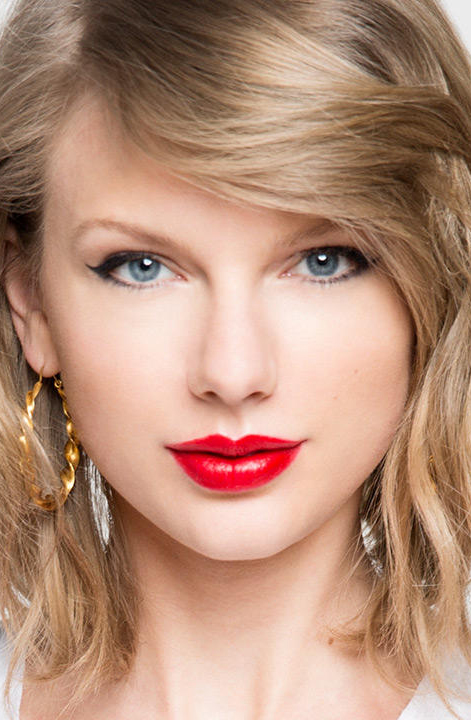
where \(t_1\) and \(t_2\) are tuples. The costs could similarly be altered to reflect the cost of each individual orientation rather than being expressed as the minimum of the two. This expansion effectively doubles the number of decision variables in the model, resulting in slower solving times. As an example, we show below a comparison of solution times for an image of Taylor Swift.
| Sets | Infer from \(c_{dp}\) | Augment \(P\) to \(\hat{P}\) |
|---|---|---|
| 18 | 11.85s | 15.94s |
| 72 | 86.32s | 211.70s |
| 162 | 349.56s | 668.46s |
With minimal additional effort, calculating the correct orientations by examining \(c_{dp}\) after the solve is strongly preferred over doubling the number of acceptable orientations.
Examples
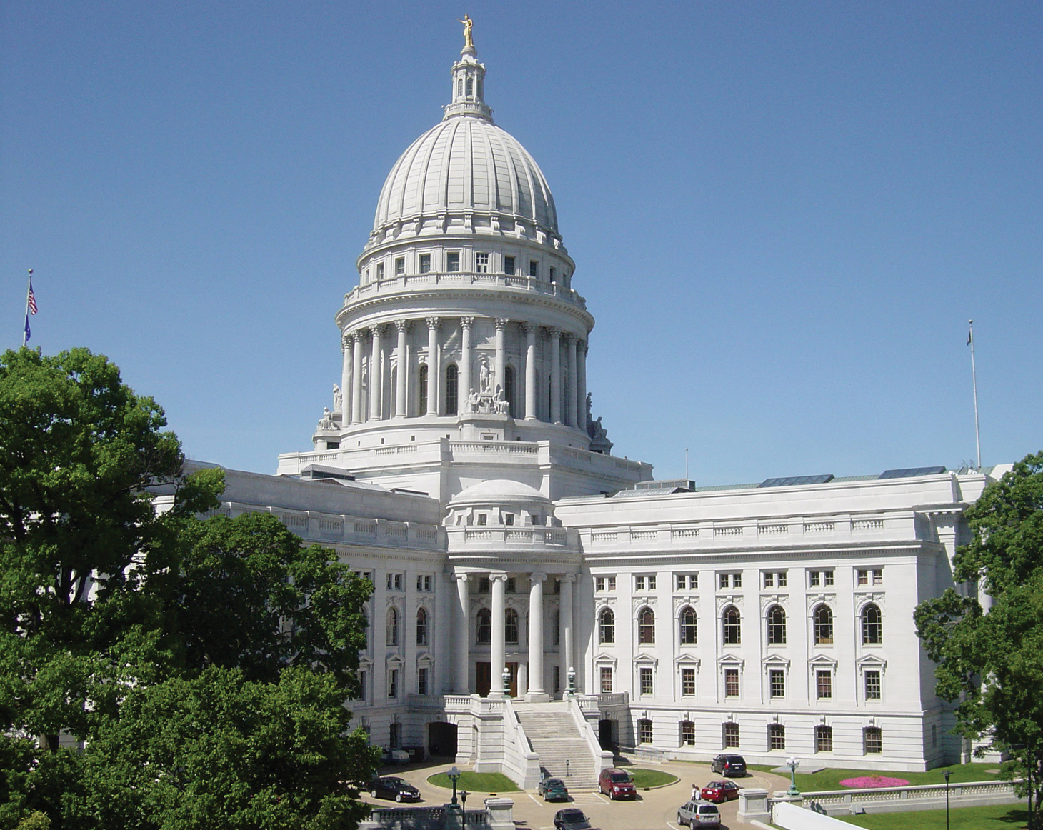
The first image is the target image and the second image is the image created by the NEOS Domino solver (using 896 complete sets of dominoes).

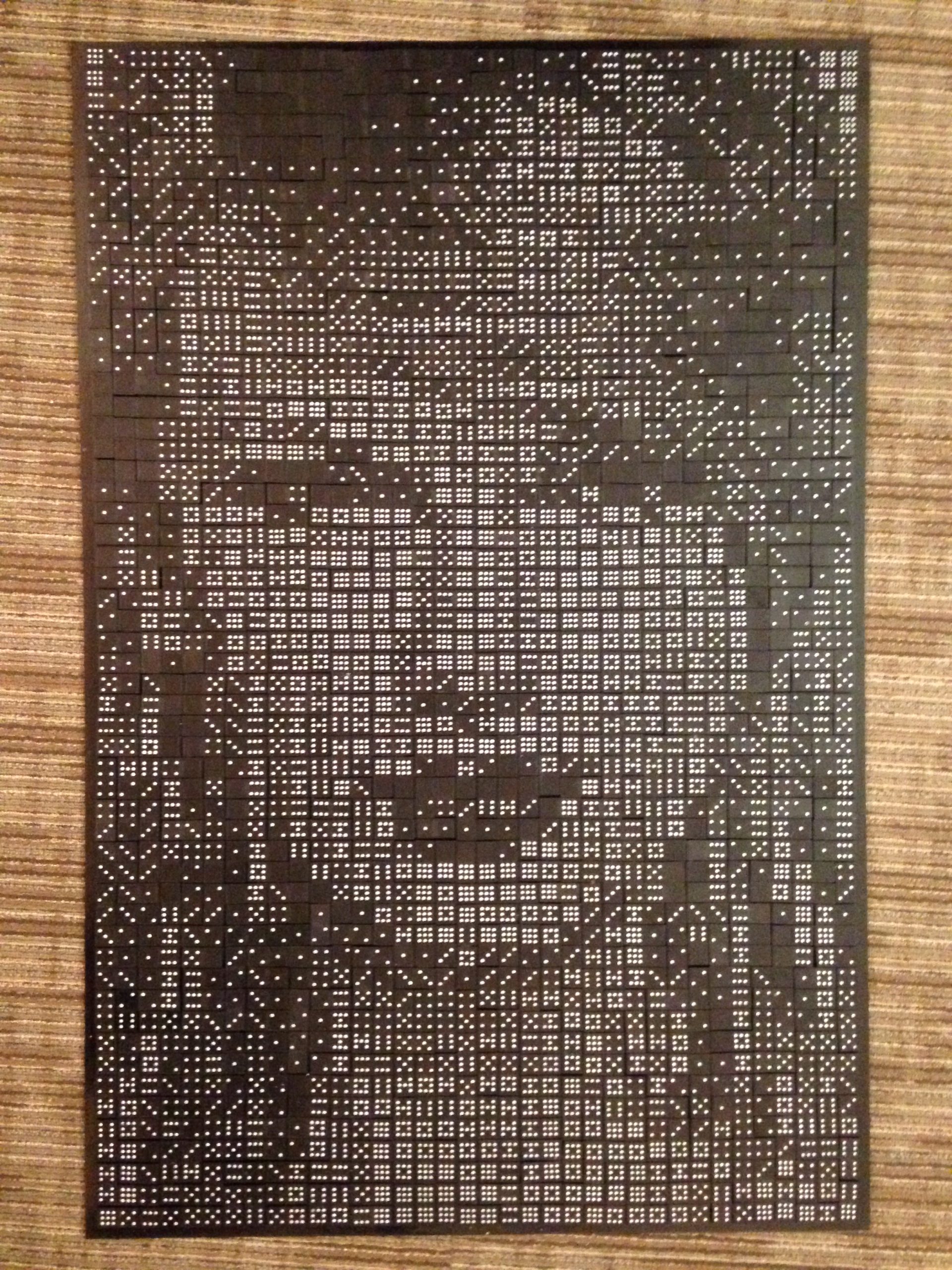
The first image is the target image of Taylor Swift and the second image is the image, created by the NEOS Domino solver, constructed in dominoes! The physical construction of the domino portrait is captured here in a time-lapse video.
Resources
- Robert Bosch’s webpage at Oberlin College
- Robert Bosch’s Domino Artwork page
- Robert Bosch’s TSP Art page