
Introduction
The design and development of efficient microbial strains for the production of everything from medicine to biofuels is an increasingly relevant and challenging problem. While the rational design of strains with desirable chemical phenotypes can be accomplished through expertise and speculation, these mutant proposals are inherently qualitative and potentially suboptimal in both the required design effort and the resulting strain performance. To refine and expedite the process of creating and evaluating mutant strains, genome-scale metabolic models, in conjunction with strain design algorithms, allow for the fast and facile quantitative generation and analysis of proposed mutants to accomplish expressed engineering objectives.
Genome-Scale Metabolic Models

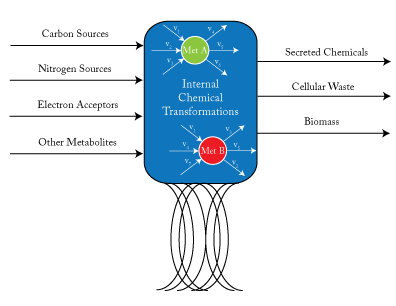
By assuming a flow balance across all nodes internal to the cell, one can solve for the steady state flux distribution within a cell. \(v_{j}\) is a reaction flux that involves met A as a product or reactant.
Genome-scale models are a mathematical recapitulation of the chemical transformations within the cell. Once all reactions within the cell have been determined, the stoichiometric coefficients are taken to populate a stoichiometric matrix, \(S_{ij}\). By convention, coefficients of reactants are written as negative values while product coefficients have a positive value.

Using this stoichiometric matrix, which can be thought of as the arcs of a network model, one can solve for the steady state behavior of the cell subject to chemical uptake and secretion (which can be considered respectively the source and sink nodes of the network). From a physical perspective, this amounts to applying the law of conservation of mass to the cell system while assuming no material accumulation. This can be written as:
\(S_{ij}v_{j}=0 \quad \forall j \in Metabs \quad [Steady~State~Material~Balance] \)
using Einsteinian notation.
To solve this particular problem, a toy model of “Escherichia coli” metabolism described by Palsson[1] was used and modeled, for simplicity, assuming growth in glucose minimal media. This model contains only a fraction of the reactions and genes that would be found in more sophisticated “E. coli” models such as the iJR904 [2] or iAF1260 [3] models. Additionally, this model does not take into account regulatory effects.
Gene to Protein to Reaction Associations (GPRs)
Genes and the protein products they code for determine the reaction network of a cell. In order to make informed decisions about the behavior of cells and their mutant strains, one must first understand the function of their genes.
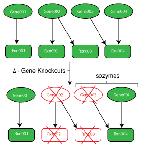
While the metabolic model is valuable for predicting phenotypic behavior of a single wild type strain, designing an efficient strain (i.e. removing reactions) requires knowledge of the functions of the cell’s numerous genes. To incorporate this knowledge into the models, mappings are made from genes to their proteins to the reactions they catalyze. These maps are commonly referred to as gene to protein to reaction associations (GPRs). Using binary variables, it is possible to model gene loss within the model and cascade the impact of this occurrence to the reaction level.
A gene’s proteins may have a number of functions and interactions within the cell. A number of relevant phenomena (as they relate to metabolic strain design) include:
- One-to-One Interaction: The simplest of interactions. A single gene is associated with a single reaction and vice versa.
- Isozymes: Multiple enzymes exist to perform a specific function. This often will require multiple gene deletions to remove the particular function from the cell.
- Multi-functional Protein: Protein is responsible for catalyzing multiple, although often, related reactions.
- Subunits: Multiple proteins (subunits) are required to create the final functional protein. The deletion of any of the genes related to this protein removes the related reaction.
While outside the scope of this problem, an additional layer of complexity can be added by modeling the impact of genetic regulation using various transcription factor (TF) rules. This is accomplished using integrated metabolic and regulatory models.
Flux Balance Analysis (FBA)
Flux balance analysis allows one to ascertain the maximal feasible reaction flux that a cell could produce given a set of media conditions and flux constraints. The model system is interrogated via FBA using an LP of the following form:

A common assumption in solving for flux distributions is that adaptive evolutionary strains will work to fulfill their biological imperative (i.e., their objective is to propagate to perpetuate their genetic code) [4]. This objective is modeled using a unique reaction flux, the biomass reaction, commonly written as \(\mu\) or \(v_{Bio}\), that behaves as a sink for the network.
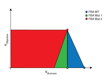
Circles represent the resulting FBA
Flux Variability Analysis (FVA)
Flux variability analysis allows one to determine if multiple flux distributions exist for a particular optimal solution [5]. For the purposes of this problem, FVA is used to generate the feasible space for the strain’s chemical production vs. biomass production. FVA is an LP of the following form:

where \(x\) is a parameter used to set biomass production along a point in its domain and \(R\) and \(M\) are sets as defined above. For this particular problem, \( c_{j} = 0 \quad \forall j \in R \backslash COI \) and \( c_{COI} = 1\). For each point along the domain, the maximum and minimum flux values for the chemical of interest are determined. The resulting figure is effectively a cross-section of the convex hull. Within this region, FBA will always select the flux distribution associated with the rightmost extreme point. If this distribution does not have a unique chemical phenotype, the maximum potential production value will be reported.
Simplified OptOrf Strain Design Algorithm
OptOrf is a bilevel mixed integer linear programming (MILP) strain design algorithm developed by Kim and Reed[6]. The algorithm works to maximize the production of a user specified chemical subject to the assumption of maximal cellular growth (i.e., it should be predictive of adaptive evolutionary strains). The MILP is implemented as described below:

Notation
- \( \Delta \) is a user-specified parameter limiting the number of gene deletions allowed.
- \( \Delta’ \) is a user-specified parameter mandating a minimum number of gene deletions by the algorithm.
- \( \delta \) is a user-specified penalty for gene deletions
- \( a_{j} \) is a reaction decision variable (binary) that indicates whether a reaction is present
- \( ko_{g} \) is a gene knockout decision variable. \(ko_{g} \in \{0,1\} \)
- \(GPR_{j,n,g}\) is the set of gene, isozyme, and reactions pairs \( \in \{R \times N \times G \}\) where \(N\) is the set of isozyme numbers \((|N| = \max_{j}\) # of isozymes for \(rxn_{j})\) and \(G\) is the set of all genes.
- \(Isozyme_{j,n}\) is a binary decision variable that indicates the expression of a gene and, thus, the presence on an enzyme
- \(\pi\) is a Relational Projection Operator
The final three constraints are rules used to map a gene deletion down to the reaction level using the GPR mappings provided to the model. For this problem, \( c_{j}v_{j} = v_{COI} \).
Interactive Demo
The objective is to produce a chemical in E coli. The user can specify a set of genes to knock out in trying to produce the selected chemical. The user-generated knockout solution is compared to the wild type (no knockouts) solution and the optimal OptORF solution.
- Select the target chemical from the drop down menu.
- In the genes table, click “Select” to select a gene to knock out in the user-generated solution.
- Set the parameters for the OptORF model by specifying the penalty for deleting a gene, the minimum number of gene deletions and the maximum number of gene deletions. Click “Aerobic” to specify aerobic conditions.
- Click on “Solve with NEOS” to generate the user-generated solution, the wild type solution, and the optimal OptORF solution. Note that there may be a minute or two before the results table and the graphs appear.
The results contain the FBA predicted secretion rate of the selected chemical [mmol/(gDW*hr)] and the cellular growth rate [1/hr] for the Wild Type (WT), User Designed (User) and OptOrf designed strains. The graphs outline the feasible set of solutions (growth and chemical production phenotypes) for each of the three strains based on FVA. This is effectively a cross-section of the cell’s solution space polytope.
Select genes to “knock out” in the user-generated solution.
Set parameters for the OptORF model.
- Gene deletion penalty
- Minimum number of gene deletions
- Maximum number of gene deletions
Select conditions
- Aerobic
References
- Palsson, B.O. 2006. Systems Biology: Properties of Reconstructed Networks. Cambridge University Press, New York.
- Reed, J.L., T.D. Vo, C.H. Schilling, and B.O. Palsson. 2003. An expanded genome-scale model of Escherichia coli K-12 (iJR904 GSM/GPR). Genome Biology, 4(9), R54.1 – R54.12.
- Feist, A.M., C.S. Henry, J.L. Reed, M. Krummenacker, A.R. Joyce, P.D. Karp, L.J. Broadbelt, V. Hatzimanikatis, and B.O. Palsson. 2007. A genome-scale metabolic reconstruction for Escherichia coli K-12 MG1655 that accounts for 1260 ORFs and thermodynamic information. Molecular Systems Biology, 3:121.
- Orth, J.D., I.Thiele, and B.O. Palsson. 2010. What is flux balance analysis? Nat Biotech, 28(3), 245-248.
- Reed, J.L. and B.O. Palsson. 2004. Genome-Scale in Silico Models of E. coli Have Multiple Equivalent Phenotypic States: Assessment of Correlated Reaction Subsets That Comprise Network States. Genome Research, 14(9), 1797-1805.
- Kim, J. and J.L. Reed. 2010. OptORF: Optimal metabolic and regulatory perturbations for metabolic engineering of microbial strains. BMC Systems Biology, 4:53.