
This Enzyme Cost Minimization case study describes the optimization of a metabolic network and uses the ECM solver to process the models. After reading through this case study, if you wish to process your own data using the NEOS server, the following three data input formats are available:
Introduction
Flux distributions of maximal growth rate (or maximal enzyme-specific biomass production) can be found by screening all elementary flux modes (EFMs) in a given model. For each EFM, the enzyme cost, which is the sum of necessary enzyme concentrations or mass concentrations, is computed by solving a convex optimality problem. If we scale all EFMs to a standard biomass production rate of 1, we directly obtain the specific enzyme cost — the enzyme cost per biomass production. From this cost, we compute the corresponding cell growth rate. A linear formula can be derived by assuming that the enzymes described in our model comprise a fixed fraction (about one eighth) of the dry weight; half of the cell’s dry weight is protein and the metabolic enzymes comprise about 25% of all proteins. An alternative nonlinear formula can be derived; it accounts for the fact that the fraction of metabolic enzymes in the proteome decreases with the growth rate — at least if the growth rate changes are due to metabolic efficiency, e.g., due to nutrient types, nutrient levels, or dilution in chemostats. Screening the EFMs corresponds to an exhaustive screening of all fluxes. If we take the convex hull of EFMs in the rate-yield spectrum, the image of the actual set of all flux distributions would be enclosed in it. For each condition (a set of given enzyme parameters and external concentrations), the EFMs with the highest predicted growth rate can be determined, and trade-offs between growth and yield can be assessed by inspecting the Pareto front. The predicted enzyme demand depends on all parameters of the kinetic model, such as external glucose or oxygen supply. By varying these parameters and repeating the calculation, we can determine how the choice of optimal fluxes depends on conditions.
Method
The optimization of a metabolic network is complicated by the fact that the conversion of one metabolite into another by an enzyme follows nonlinear dynamics. Many tools can optimize linear properties of a metabolic network but the tool described here optimizes the complete metabolic network including the kinetics of the metabolite conversions. Optimizing a kinetic network is a balance between investment (enzymes) and the reward (production of the target metabolite / biomass). In effect, the problem is to optimize the specific objective flux, which is the ratio defined as:
$$\frac{\text{objective flux}}{\text{total enzyme investment}}$$
The tool maximizes the specific objective flux by minimizing the investment for a given objective flux. In a network without additional constraints, the flux distribution that maximizes the specific objective flux is always an EFM ([1] and [2]), so therefore it is sufficient to optimize for all EFMs to find the optimal enzyme investment. The tool can be used to optimize any flux distribution, e.g. a measured rate distribution.
The use of the tool will be explained with a toy model:
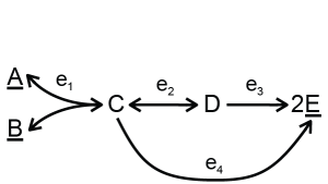
Two different versions of input can be used to describe the network and kinetics — separate files or a single file. The structure of the network is described in the stoich file/table, where the reactions are named with identifiers. In the case of the toy model, the reactions catalyzed by enzymes \(e_1, e_2, e_3\) and \(e_4\) are named R1, R2, R3 and R4 respectively. The kinetics of all reactions are specified in a number of files/tables. The easiest way it to use modular rate laws [3] for all reactions. For example, for a reaction A + B -> C, the rate equation would be:
$$\frac{E \cdot k_{cat} (\frac{A}{K_{MA}} \cdot \frac{B}{K_{MB}})}{(1 + \frac{A}{K_{MA}})(1 + \frac{B}{K_{MB}})+(1+\frac{C}{K_{MC}})-1}$$
Using this rate equation, only the \(K_M\) values and \(k_{cat}\) values for all the reactions need to be specified. The \(K_M\) values need to be specified for all metabolites involved in the reaction as well as for the products. Reversible reactions are determined by an existing \(K_{eq}\) for that reaction. There is no need to specify a reverse \(k_{cat}\) since that is then determined by the Haldane relationship. Concentrations for the external metabolites need to be given, and if a metabolite has the value 0, eps is used instead of a value.
As the last step, the rate distributions are optimized. The toy model has two elementary flux modes, one using R2 and R3 and one using R4, which will be optimized in this example. If we divide the flux of R1 (1) by the minimal enzyme investment of these two EFMs, we get the optimal specific flux of this network for the objective flux R1. The input files for this toy model can be downloaded in a single file or a collection of files.
Now we can get the minimal enzyme investment and the levels of the internal metabolites and enzymes using the online application ECM with single file input or ECM with zip file input. The output will include a file summary.csv with the minimal enzyme investment for each rate distributions and files enz.csv and met.csv for the individual enzyme and metabolite levels.
In the following sections, we describe several options: allosteric regulation, enzyme weights, bounds, moieties, and custom rate equations.
Allosteric regulation
The toy model can include allosteric regulation, for example:
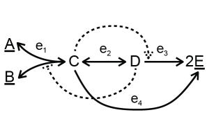
In this example, metabolite D inhibits reaction R1 and C activates reaction R3. This information can be added to the model. Using convenience kinetics, only the inhibition or activation constants need to be specified (download a single file with allosteric regulation or a collection of files with allosteric regulation). For an inhibitor, the rate equation will be multiplied by the term \(1/(1 + inh/K_i)\), where \(K_i\) is the inhibition constant. For an activator, the rate equation will be multiplied by the term \((act/K_a)/(1 + act/K_a)\) where \(K_a\) is the activation term. One rate can have multiple activation and inhibition terms or combinations of them. Other forms of inhibition and activation also can be seen in Custom rate equations below.
The tool will set an inhibitor that is not associated with any active reactions, such as inhibitor D in rate distribution 2, automatically to 0. An activator that is not associated with any active reactions (not possible in our toy model) will automatically be set equal to the activation constant, and therefore half the maximal rate for that reaction.
Enzyme weights
Some enzymes can be more costly than others. Enzyme weights can be taken from different quantities, e.g., gene length, enzyme weight or number of carbon atoms in the enzyme. In theory, the \(k_{cat}\) values can be divided by the enzyme weights to give the same solution, but it is cleaner to supply an enzyme weight file. Download a single file with weights or a collection of files with weights.
Enzyme and metabolite bounds
The enzyme levels are minimized, so in theory they should not get too high. In some cases, however, it might be necessary to add bounds such that the levels are realistic. The metabolites are more important to constrain, since the algorithm does not contain anything to ensure physiological realistic level are reached. Bounds for all enzymes and/or metabolites need to be specified when this option is used, but inf (for unbounded) can be used. Download a single file with bounds or a collection of files with bounds.
Conserved moieties
A combination of metabolites can be used but not produced by the metabolic network under study, for example, with co-factors. In some models, the concentrations of [AMP], [ADP] and [ATP] can change individually, but their sum [AMP]+[ADP]+[ATP] will always remain constant, because these metabolites are only converted into each other. There are two strategies to deal with conserved moieties: (1) the levels of these metabolites can be fixed and added to the fixed metabolites or (2) the total of these metabolites can be fixed, because the metabolic network under study can affect the ratio of these metabolites in some cases. In the second strategy, these so-called moieties need to be defined. For example, consider the following network:
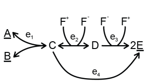
The total of F+ and F- cannot be altered by this metabolic network. To keep the total constant at some measured value, the following files can be used: a single file with a conserved moiety or a collection of files with a conserved moiety.
Custom rate equations
For the basic rate equations, we only need to supply the \(K_M\) values and \(k_{cat}\) values. However, some enzymes are known to use other kinetics. Because the internal calculations use a very general format for the rate equation, most rate equations can be incorporated, although some preprocessing might be necessary. The general formula looks like [4]:
$$v = e \cdot k_{cat,f} \cdot \eta^{th} \cdot \eta^{kin}$$
$$\eta^{th} = 1 – K_{eq}^{-1} \cdot e^{-n*x}$$
$$\eta^{kin} = (\sum_k α_k \prod_j c_j a_{jk})^{-1}$$
with \(c_j\) the metabolite concentrations. The index \(k\) runs over the terms in the kinetic term and \(j\) over the substrates. To use this formula, the \(k_{cat}\) must be provided but the \(K_{eq}\) is optional (if not provided, \(ƞ^{th}\) is set to 1). Instead of the \(K_M\), the sets \(a\) and \(α\) must be provided. The set \(n\) is taken from the stoichiometries. Download the input files for the toymodel with the sets \(a\) and \(α\) instead of \(K_M\) values in a single file or a collection of files .
This option can be used to implement a Hill equation:
$$v_3 = e_3 \cdot k_{cat,3} \cdot \frac{D^{1.4}}{(K_{0.5}^{1.4} + D^{1.4})}$$
The fraction in the rate equation needs to be rewritten such that there is a 1 in the numerator:
$$\frac{D^{1.4}}{K_{0.5}^{1.4} + D^{1.4}} = \frac{1}{\frac{K_{0.5}^{1.4}}{D^{1.4}} + 1}$$
There are two terms in the denominator. Therefore, we have \(k=1\) and \(k=2\). The value of \(α_2\) is 1 and all of the \(a_{j,2}\) terms are 0 (we do not have to provide them). The term \(α_1\) is \(K_{0.5}^{1.4}\) and all of the \(a_{j,1}\) terms are 0 except for \(a_{D,1}\), which is -1.4. Download a single file with a hill equation or a collection of files with a hill equation.
Custom rate equations also can be used to include different types of allosteric regulation.
Application of the algorithm
The algorithm can be applied to a model of the central carbon metabolism of E. coli [5]. Under aerobic conditions, this model contains 687 EFMs that produce biomass.
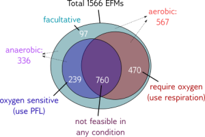
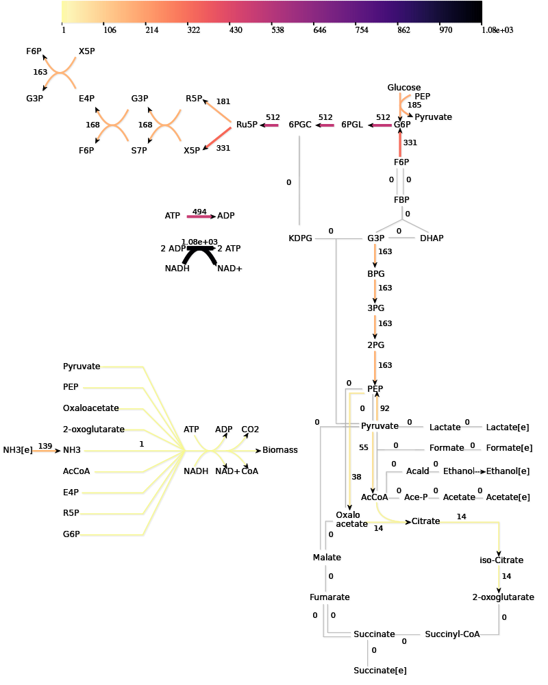
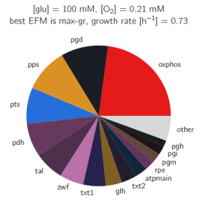
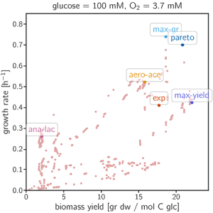
The paper gives many examples of how the growth optimization data can be used, but the main aim was to investigate a trade-off between growth and yield. The algorithm can be used to plot the rate and yield of all the EFMs. To obtain the optimal enzyme levels, we run this Ecoli.zip input file. The yield \(Y_{g/C})\ and growth rate\(\mu\) are calculated with the following formulas:
$$\mu = \frac{0.135 \cdot \frac{7.44*10^7}{\sum_i (e_i W_i)}}{1 + 0.1 \cdot \frac{7.44 \cdot 10^7}{ \sum_i (e_i W_i)}}$$
$$Y_{g/C} = 20666 v_{biom} / 6 v_{pts}$$
The plotting of the data gives the following figure:
Interactive Demo
In this section, the user can investigate how changes in the initial conditions affect growth rates. Five EFMs and the wild type flux distribution are selected for the demo. (See Fig. 5 and Table 1 in mM
oxygen
mM
glucoseExt
mM
\(k_{cat,Biomass}\)
\(s^{-1}\)
\(k_{cat,TPI}\)
\(s^{-1}\)
\(k_{cat,OXphos}\)
\(s^{-1}\)
Results
| EFM name | Yield (g/mol-C) | Old Growth Rate (\(h^{-1}\)) | New Growth Rate (\(^{-1}\)) |
|---|---|---|---|
| max-gr (1565) | 18.6 | 0.739 | |
| max-yield (938) | 22.1 | 0.422 | |
| ana-lac (1295) | 2.07 | 0.258 | |
| pareto (1218) | 20.8 | 0.699 | |
| aero-ace (559) | 15.8 | 0.520 | |
| exp (9999) | 17.7 | 0.409 |
For more information on Enzyme Cost Minimization including MATLAB code and Python code, please visit the Enzyme Cost Minimization website.
References
- Wortel, Meike T., Han Peters, Josephus Hulshof, Bas Teusink, and Frank J. Bruggeman. “Metabolic states with maximal specific rate carry flux through an elementary flux mode.” FEBS Journal 281, no. 6 (2014): 1547-1555. https://doi.org/10.1111/febs.12722
- Muller, Stefan, Georg Regensburger, and Ralf Steuer. “Enzyme allocation problems in kinetic metabolic networks: Optimal solutions are elementary flux modes.” Journal of Theoretical Biology 347 (2014): 182-190. http://dx.doi.org/10.1016/j.jtbi.2013.11.015
- Liebermeister, Wolfram, Jannis Uhlendorf, and Edda Klipp. “Modular rate laws for enzymatic reactions: thermodynamics, elasticities and implementation.” Bioinformatics 26, no. 12 (2010): 1528-1534. https://doi.org/10.1093/bioinformatics/btq141
- Noor, Elad, Avi Flamholz, Arren Bar-Even, Dan Davidi, Ron Milo, and Wolfram Liebermeister. “The protein cost of metabolic fluxes: prediction from enzymatic rate laws and cost minimization.” PLoS Comput Biol 12.11 (2016):e1005167. https://doi.org/10/1371/journal.pcbi.1005167
- Wortel, Meike T., Elad Noor, Michael C. Ferris, Frank J. Bruggemann, and Wolfram Liebermeister. “Profiling metabolic flux models by enzyme cost reveals variable trade-offs between growth and yield in Escherichia coli.” bioRxiv (2017):111161. https://doi.org/10.1101/111161